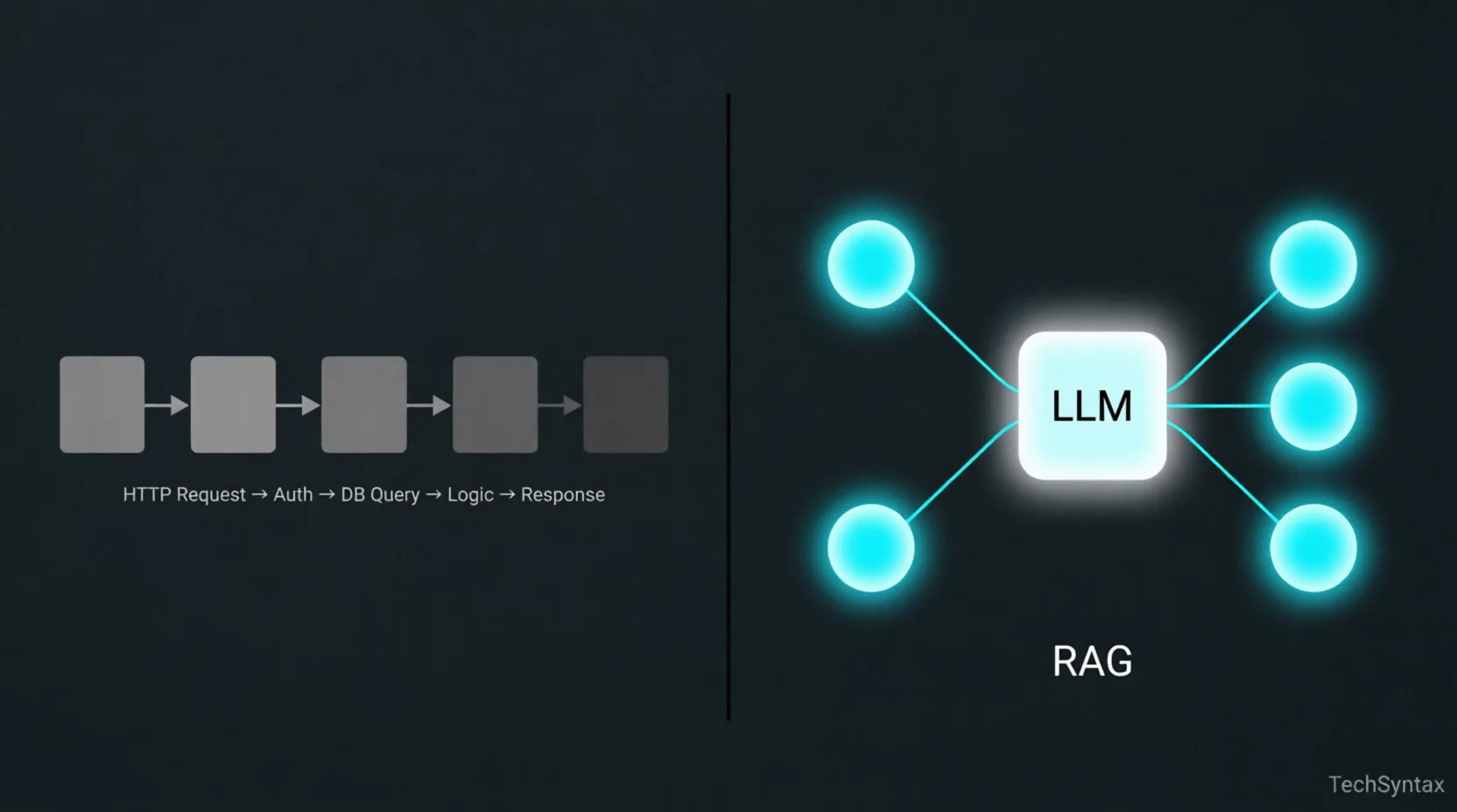

Traditional API vs. RAG
A minimalist comparison showing the linear nature of traditional APIs versus the retrieval-based nodes of a RAG pipeline.
RAG Systems for Backend Devs: How They Actually Work
Everyone talks about RAG like it's magic. You plug in your documents, and suddenly your LLM "knows" your data. But if you've tried building one in production, you know that's not how it goes. Retrieval breaks. Context gets bloated. Responses degrade in unpredictable ways. Latency spikes under load.
This article is not a tutorial. It's an engineering explanation — what actually happens inside a RAG pipeline, where each layer can fail, and how to reason about it as a backend developer already comfortable with APIs, databases, and distributed systems.
What is RAG (Retrieval-Augmented Generation)?
RAG is a pattern where an LLM's response is grounded by dynamically retrieved documents injected into its prompt at inference time. Instead of relying solely on the model's training data, the system fetches relevant context from an external store — typically a vector database — and appends it to the user's query before sending it to the model. The model never "learns" your data; it reads it freshly on every request.
The Real Problem RAG Solves (It's Not What You Think)
The common framing is: "LLMs have a knowledge cutoff, so RAG keeps them up to date." That's partially true, but it's the least interesting reason to use RAG.
The deeper problem RAG solves is specificity at inference time. A general-purpose LLM knows roughly everything and specifically nothing about your domain. Your internal HR policies, your banking product rules, your customer contracts — none of that is in the model's weights. You can't prompt-engineer your way to specificity when the knowledge doesn't exist in the model.
Fine-tuning is the obvious alternative. But fine-tuning bakes knowledge into weights at training time. That means every update to your data requires a retraining cycle. For backend systems dealing with frequently changing data — policy documents, product catalogs, support tickets — RAG wins decisively on operational grounds alone.
RAG lets you treat the LLM as a reasoning engine and your document store as the knowledge layer. That separation of concerns is what makes it architecturally interesting to backend engineers.
The RAG Pipeline as a Backend Engineer Sees It
Strip away the AI branding and RAG is a pipeline with two distinct phases: an indexing phase (offline) and a retrieval phase (online, per-request). Most production issues come from conflating the two or failing to design them independently.
Phase 1: Indexing (Offline)
- Load raw documents (PDFs, HTML, Markdown, database rows)
- Split documents into chunks using a chunking strategy
- Run each chunk through an embedding model to get a float vector
- Store the vector + chunk text + metadata in a vector database
Phase 2: Retrieval + Generation (Online, Per-Request)
- Receive the user query
- Embed the query using the same embedding model used at indexing
- Run an ANN (approximate nearest neighbor) search against the vector store
- Retrieve top-K chunk texts by cosine similarity score
- Assemble a prompt: system instructions + retrieved chunks + user query
- Send the prompt to the LLM and stream the response
The indexing phase is essentially a batch ETL job. The retrieval phase is a latency-sensitive API call. Design them with that mental model and most architectural decisions become obvious.
Embeddings: What's Actually Happening Under the Hood

RAG Architecture Flow
Top-down data flow: Query → Embedder → Vector DB (HNSW) → Retrieval → Prompt Assembly → LLM → Response.
An embedding model transforms text into a high-dimensional float vector — typically 768 to 3072 dimensions depending on the model. The key property: semantically similar texts produce vectors that are geometrically close in that high-dimensional space.
This is not keyword matching. "Payment failed" and "transaction declined" will be close in embedding space even though they share no tokens. That's the entire value proposition.
What backend engineers need to understand:
- Embedding models are neural networks. They have inference latency (10–80ms per call depending on model size and hardware). Batching is essential at indexing time.
- Model version pinning matters. If you re-index with a different embedding model version, your old stored vectors are invalid. The query embedding and stored embeddings must come from the same model.
- Max token limits apply. Most embedding models have a max input of 512 or 8192 tokens. Text beyond that is silently truncated or throws an error. Your chunking strategy must respect this ceiling.
- Dimensionality affects storage and search cost. A 3072-dimensional vector for 10 million chunks requires significant memory in your vector index. This is a real infra planning concern.
Popular embedding models in production today:
| Model | Dimensions | Max Tokens | Notes |
|---|---|---|---|
| text-embedding-3-small (OpenAI) | 1536 | 8191 | Good default. Cost-efficient. |
| text-embedding-3-large (OpenAI) | 3072 | 8191 | Higher quality, 2× storage cost. |
| nomic-embed-text (local) | 768 | 8192 | Self-hostable. Good for private data. |
| bge-large-en-v1.5 (HuggingFace) | 1024 | 512 | Strong benchmark scores. Short context. |
Vector Search Internals: Why It's Fast and Where It Lies
Exact nearest-neighbor search over millions of vectors with 1536 dimensions is computationally prohibitive at query time. Vector databases solve this with ANN (Approximate Nearest Neighbor) algorithms — HNSW (Hierarchical Navigable Small World) being the most common in production systems like Qdrant, Weaviate, and pgvector.
HNSW builds a multi-layer graph structure over your vectors at index time. At query time, it traverses this graph starting from a random entry point, greedily moving toward neighbors closer to the query vector. It's fast because it never compares against every vector — it prunes the search space aggressively using the graph structure.
The trade-off: it's approximate. It may miss the truly closest vector if that vector is in an unexplored graph region. You tune the recall/speed trade-off with parameters like ef_construction (index-time quality) and ef (query-time quality). Most production systems run at ~95% recall — good enough, but you should know it's not exact.
What this means practically:
- Vector search latency is typically 2–15ms for well-tuned indexes with millions of vectors.
- Memory is the constraint, not CPU. HNSW indexes are RAM-resident. A million 1536-dim vectors ≈ ~6GB RAM for the index alone.
- Index build time grows non-linearly. Re-indexing 50M documents is a multi-hour operation. Design incremental upsert flows, not full rebuilds.
Chunking Strategies: The Underrated Core Decision
Chunking is where most RAG implementations silently degrade. The embedding model compresses your chunk into a single vector. The quality of that compression depends entirely on whether the chunk contains a coherent, self-contained unit of meaning.
A chunk that spans two unrelated topics will produce an ambiguous vector that ranks poorly for both. A chunk that's too short loses context. A chunk that's too long dilutes the signal.
| Strategy | How It Works | Best For | Watch Out For |
|---|---|---|---|
| Fixed-size (token count) | Split every N tokens with optional overlap | Uniform content (logs, records) | Cuts mid-sentence; kills coherence |
| Sentence-based | Split on sentence boundaries | Narrative text, articles | Individual sentences often lack context |
| Recursive character split | Split by paragraph → sentence → word | General documents | Default LangChain behavior; reasonable baseline |
| Semantic chunking | Embed each sentence; split where cosine similarity drops | Mixed-topic documents | Expensive at indexing; double embedding cost |
| Document-aware (Markdown, HTML) | Split on headings/sections | Structured docs, wikis, API docs | Requires format-specific parsers |
In a project involving a large policy document corpus, we started with fixed-size 512-token chunks and hit a wall: answers were partial and contextually wrong. Switching to document-aware splitting (by heading hierarchy) with a 20% overlap window cut hallucination rate significantly and improved user-rated answer quality. The chunk size wasn't the issue — the semantic integrity of each chunk was.
Practical defaults to start with:
- Chunk size: 256–512 tokens
- Overlap: 10–20% of chunk size
- Always include document title and section heading as chunk metadata (prepend to chunk text or store as filterable field)
Context Injection: The Prompt Assembly Layer
After retrieval, you have your top-K chunks. Now you need to construct the prompt. This layer is surprisingly consequential and often treated as an afterthought.
A typical RAG prompt structure:
System:
You are a helpful assistant. Answer questions based strictly on the context below.
If the answer is not in the context, say you don't know.

Context:
---
[Chunk 1 text]
Source: policy-handbook.pdf, Section: Leave Policy
---
[Chunk 2 text]
Source: policy-handbook.pdf, Section: Sick Leave
---

User Query:
How many sick days am I entitled to per year?
Key decisions at this layer:
- How many chunks (K)? More chunks = more context = better coverage. But LLMs degrade with very long contexts (the "lost in the middle" problem — information in the center of a long context is recalled less reliably than information at the edges). Start with K=3–5.
- Include source metadata? Yes — always. It enables the model to reason about provenance and helps you debug retrieval failures. It also enables citation in the response.
- Score threshold filtering: Don't inject chunks with a similarity score below a cutoff (~0.70 cosine similarity). Low-score chunks inject noise. Better to return "I don't have information on this" than a hallucination built on a weakly relevant chunk.
- Deduplicate before injection: Near-duplicate chunks from overlapping document sections will waste context window tokens. Run a similarity check on retrieved chunks before assembling the prompt.
Where RAG Fails in Production (And Why)
These are the failure modes that don't show up in demos but hit you in real deployments.

Internal Mechanism: Chunk & Retrieve
Left: Document chunking and vector embedding. Right: Query vector plotting and nearest neighbor retrieval in 2D space.
1. Retrieval Misses the Right Chunk
Symptom: The answer is in your documents but the LLM says it doesn't know.
Root Cause: The user's query language doesn't semantically overlap with how the document is written. A user asks "Can I work from home?" but the policy document says "Remote work eligibility." These are similar in meaning but may be far apart in embedding space depending on the model.
Fix: Implement HyDE (Hypothetical Document Embeddings) — ask the LLM to generate a hypothetical answer to the query, then embed that hypothetical answer for retrieval instead of the raw query. Alternatively, use query expansion: generate 3–5 paraphrases of the query and union the retrieval results.
2. Chunk Boundary Cuts Answers in Half
Symptom: The retrieved chunk contains partial information — the answer continues in the next chunk, which wasn't retrieved.
Root Cause: Fixed-size chunking with insufficient overlap.
Fix: Increase overlap, or implement a parent-child chunk strategy: embed small child chunks for precision retrieval, but inject their parent chunk (larger context window) into the prompt. This gives you retrieval precision without context truncation.
3. Stale Index After Document Updates
Symptom: RAG answers based on outdated policy or deleted content.
Root Cause: No synchronization between the source document store and the vector index.
Fix: Treat the vector index as a derived store. Build an event-driven pipeline: document create/update/delete events trigger re-indexing of affected chunks. Store document hash + last_indexed_at metadata in the vector store for auditability.
4. Context Window Overflow
Symptom: API errors, or responses that abruptly cut off.
Root Cause: Retrieved chunks + system prompt + user query exceed the model's context limit.
Fix: Measure total token count before sending the request. Trim or re-rank chunks by relevance score and drop the lowest-scoring ones until you're within budget. Never hard-code K=5 without a token budget check.
5. Embedding Model Drift
Symptom: Retrieval quality suddenly degrades after an infrastructure update.
Root Cause: The embedding model version changed (e.g., OpenAI silently updated an endpoint, or you switched providers). Stored vectors no longer align with query vectors from the new model.
Fix: Version-pin your embedding model. When you must upgrade, run a full re-index. Treat the model name + version as a dependency in your vector store schema.
RAG vs Fine-Tuning: The Decision Is Simpler Than You Think
| Factor | Use RAG | Use Fine-Tuning |
|---|---|---|
| Data changes frequently | ✅ Yes | ❌ No |
| Need to cite sources | ✅ Yes | ❌ Hard to do reliably |
| Teaching the model a new task style | ❌ Not ideal | ✅ Yes |
| Domain-specific vocabulary/tone | ❌ Inconsistent | ✅ Yes |
| Large private document corpus | ✅ Yes | ❌ Expensive, slow to update |
| Reducing hallucination on known facts | ✅ Yes (with grounding) | ⚠️ Partial |
| Low operational overhead | ⚠️ Requires vector infra | ⚠️ Requires training infra |
In most production backend use cases — knowledge bases, document Q&A, support automation — RAG is the right call. Fine-tuning is a tool for behavior and style, not for knowledge injection.
A Minimal RAG Implementation to Reason From
This isn't a copy-paste tutorial. It's a skeleton to make the architecture concrete.
# --- INDEXING PHASE (run offline / on document change) ---

from openai import OpenAI
import qdrant_client

client = OpenAI()
qdrant = qdrant_client.QdrantClient("localhost", port=6333)

def index_document(doc_id: str, text: str, metadata: dict):
    chunks = chunk_text(text, max_tokens=400, overlap=80)
    for i, chunk in enumerate(chunks):
        response = client.embeddings.create(
            model="text-embedding-3-small",
            input=chunk
        )
        vector = response.data[0].embedding
        qdrant.upsert(
            collection_name="documents",
            points=[{
                "id": f"{doc_id}_{i}",
                "vector": vector,
                "payload": {"text": chunk, **metadata}
            }]
        )


# --- RETRIEVAL + GENERATION PHASE (per user request) ---

def answer_query(user_query: str) -> str:
    # 1. Embed the query
    query_vector = client.embeddings.create(
        model="text-embedding-3-small",
        input=user_query
    ).data[0].embedding

    # 2. Retrieve top-K chunks
    results = qdrant.search(
        collection_name="documents",
        query_vector=query_vector,
        limit=4,
        score_threshold=0.70   # Drop low-confidence matches
    )

    # 3. Assemble context
    context_blocks = []
    for r in results:
        context_blocks.append(
            f"[Source: {r.payload.get('source', 'unknown')}]\n{r.payload['text']}"
        )
    context = "\n---\n".join(context_blocks)

    # 4. Build prompt + call LLM
    response = client.chat.completions.create(
        model="gpt-4o-mini",
        messages=[
            {
                "role": "system",
                "content": (
                    "Answer based strictly on the context provided. "
                    "If the answer is not in the context, say you don't know."
                )
            },
            {
                "role": "user",
                "content": f"Context:\n{context}\n\nQuestion: {user_query}"
            }
        ]
    )
    return response.choices[0].message.content
Points worth noting in this skeleton:
- The same
text-embedding-3-smallmodel is used at both indexing and query time. score_threshold=0.70prevents low-relevance chunks from polluting the context.- Source metadata is stored alongside each chunk and injected into the prompt.
- There's no token budget check here — add one in production before building the context string.
Realistic Latency Expectations

Latency Breakdown
Performance metrics showing LLM inference as the primary bottleneck (420ms) compared to embedding and retrieval steps.
A common surprise for teams shipping their first RAG API: the LLM call dominates latency so heavily that the retrieval overhead is nearly irrelevant. Here's a realistic breakdown for a well-tuned system:
| Pipeline Step | Typical Latency | Notes |
|---|---|---|
| Query embedding | 15–40ms | Depends on model size and API vs local |
| Vector search (ANN) | 2–15ms | Well-tuned HNSW at 1M+ vectors |
| Prompt assembly | <5ms | String ops; negligible |
| LLM inference (first token) | 300–800ms | The dominant cost. Streaming helps UX. |
| Total time-to-first-token | 350–850ms | P50 for a production-grade system |
Always stream the LLM response. A user can read a streaming response that starts arriving in 400ms. A blocking call that delivers the full response in 3 seconds will feel slow even if total tokens are identical.
What to Take Away
RAG is architecturally simple but operationally nuanced. The pipeline has four distinct responsibilities — chunking, embedding, retrieval, and context injection — and each one has failure modes that won't show up in a notebook demo but will bite you at scale.
As a backend developer, the mental model to carry is this:
- The indexing pipeline is a batch ETL job with a semantic dimension. Design it like one.
- The vector store is a derived cache of your document knowledge. Treat it as such — versioned, evictable, re-buildable.
- The retrieval step is a fast approximate search with tunable recall. Know your recall/latency trade-off.
- The prompt assembly is your API contract with the LLM. Token budgets, deduplication, and score thresholds belong here.
- The LLM is stateless and general-purpose. It contributes reasoning, not knowledge. Your retrieval layer provides the knowledge.
Get those five things right, and RAG stops feeling like AI magic and starts feeling like a well-engineered service — which is exactly what it should be.
Be the first to leave a comment!